python线性回归
von Libniz 人气:01线性回归
1.1简单线性回归
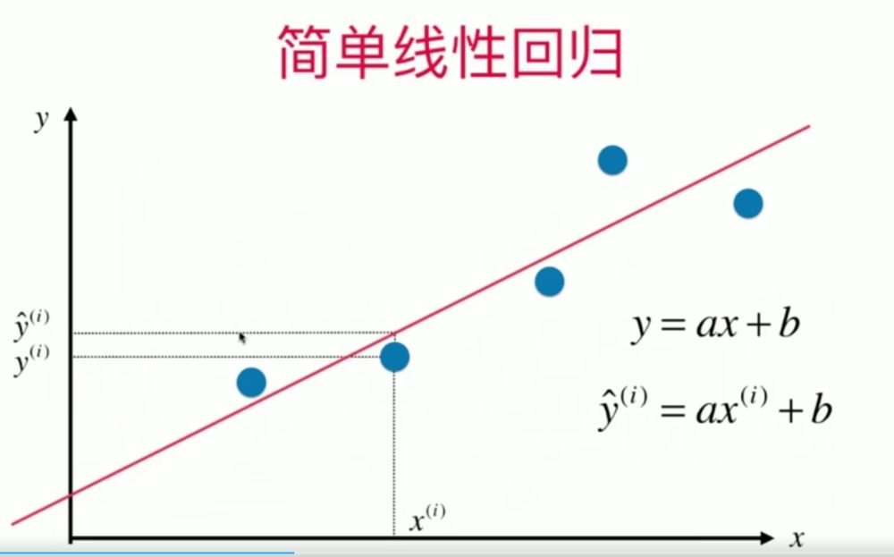
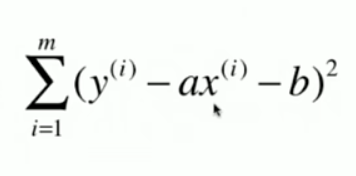
在简单线性回归中,通过调整a和b的参数值,来拟合从x到y的线性关系。下图为进行拟合所需要优化的目标,也即是MES(Mean Squared Error),只不过省略了平均的部分(除以m)。
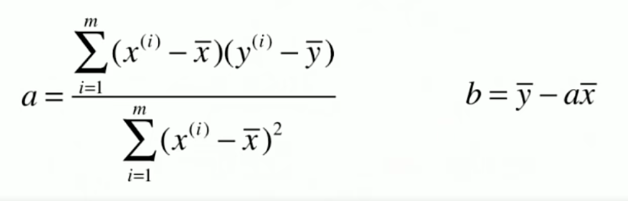
对于简单线性回归,只有两个参数a和b,通过对MSE优化目标求极值(最小二乘法),即可求得最优a和b如下,所以在训练简单线性回归模型时,也只需要根据数据求解这两个参数值即可。
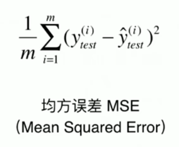
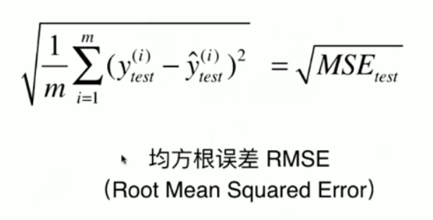
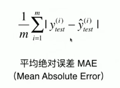
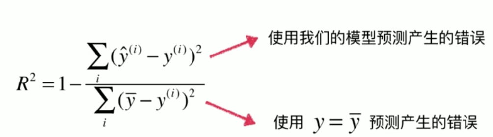
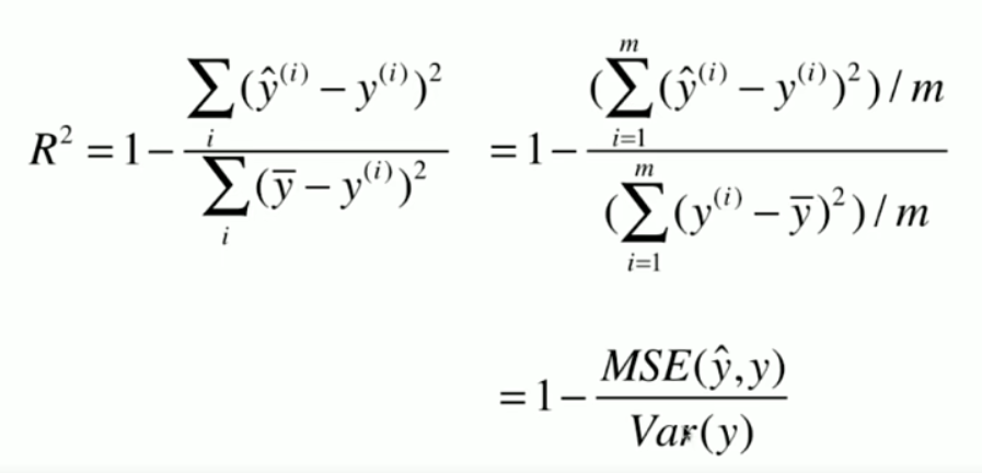
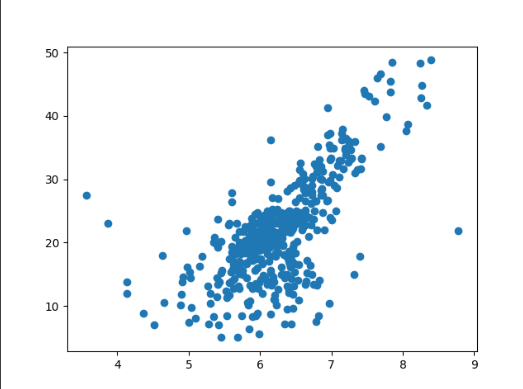
下面使用波士顿房价数据集中,索引为5的特征RM (average number of rooms per dwelling)来进行简单线性回归。其中使用的评价指标为:
# 以sklearn的形式对simple linear regression 算法进行封装
import numpy as np
import sklearn.datasets as datasets
from sklearn.model_selection import train_test_split
import matplotlib.pyplot as plt
from sklearn.metrics import mean_squared_error,mean_absolute_error
np.random.seed(123)

class SimpleLinearRegression():
    def __init__(self):
        """
        initialize model parameters
        self.a_=None
        self.b_=None
    def fit(self,x_train,y_train):
        training model parameters
        Parameters
        ----------
            x_train:train x ,shape:data [N,]
            y_train:train y ,shape:data [N,]
        assert (x_train.ndim==1 and y_train.ndim==1),\
            """Simple Linear Regression model can only solve single feature training data"""
        assert len(x_train)==len(y_train),\
            """the size of x_train must be equal to y_train"""
        x_mean=np.mean(x_train)
        y_mean=np.mean(y_train)
        self.a_=np.vdot((x_train-x_mean),(y_train-y_mean))/np.vdot((x_train-x_mean),(x_train-x_mean))
        self.b_=y_mean-self.a_*x_mean
    def predict(self,input_x):
        make predictions based on a batch of data
            input_x:shape->[N,]
        assert input_x.ndim==1 ,\
            """Simple Linear Regression model can only solve single feature data"""
        return np.array([self.pred_(x) for x in input_x])
    def pred_(self,x):
        give a prediction based on single input x
        return self.a_*x+self.b_
    def __repr__(self):
        return "SimpleLinearRegressionModel"
if __name__ == '__main__':
    boston_data = datasets.load_boston()
    x = boston_data['data'][:, 5]  # total x data (506,)
    y = boston_data['target']  # total y data (506,)
    # keep data with target value less than 50.
    x = x[y < 50]  # total x data (490,)
    y = y[y < 50]  # total x data (490,)
    plt.scatter(x, y)
    plt.show()
    # train size:(343,) test size:(147,)
    x_train, x_test, y_train, y_test = train_test_split(x, y, test_size=0.3)
    regs = SimpleLinearRegression()
    regs.fit(x_train, y_train)
    y_hat = regs.predict(x_test)
    rmse = np.sqrt(np.sum((y_hat - y_test) ** 2) / len(x_test))
    mse = mean_squared_error(y_test, y_hat)
    mae = mean_absolute_error(y_test, y_hat)
    # notice
    R_squared_Error = 1 - mse / np.var(y_test)
    print('mean squared error:%.2f' % (mse))
    print('root mean squared error:%.2f' % (rmse))
    print('mean absolute error:%.2f' % (mae))
    print('R squared Error:%.2f' % (R_squared_Error))
输出结果:
mean squared error:26.74
root mean squared error:5.17
mean absolute error:3.85
R squared Error:0.50
数据的可视化:
1.2 多元线性回归
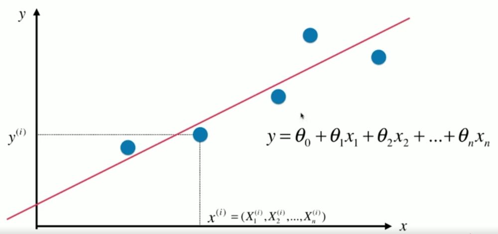
多元线性回归中,单个x的样本拥有了多个特征,也就是上图中带下标的x。
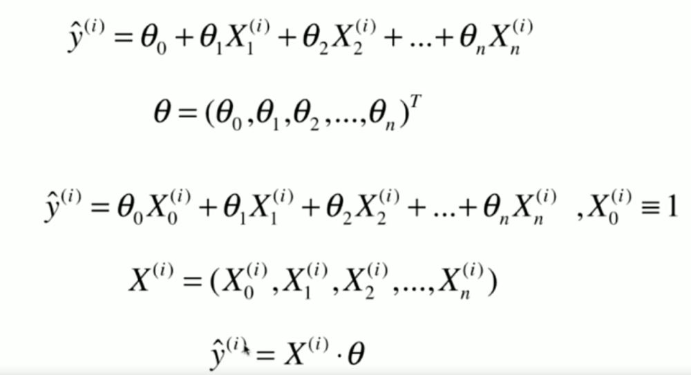
其结构可以用向量乘法表示出来:
为了便于计算,一般会将x增加一个为1的特征,方便与截距bias计算。
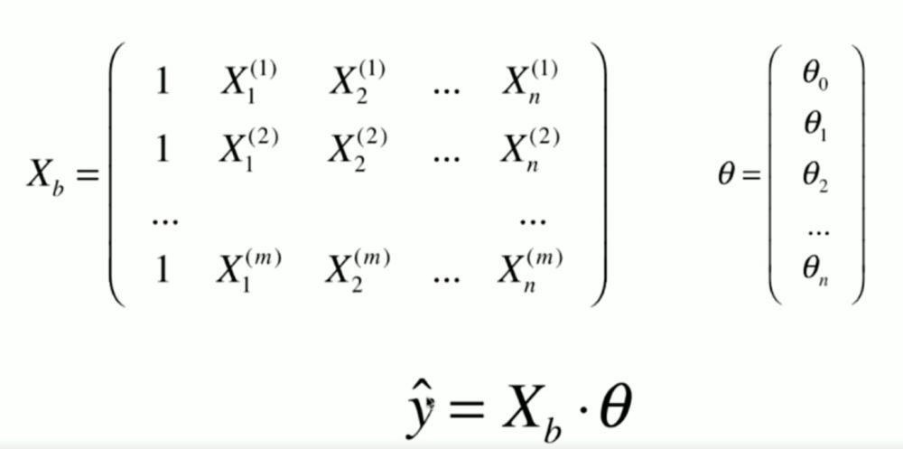
而多元线性回归的优化目标与简单线性回归一致。
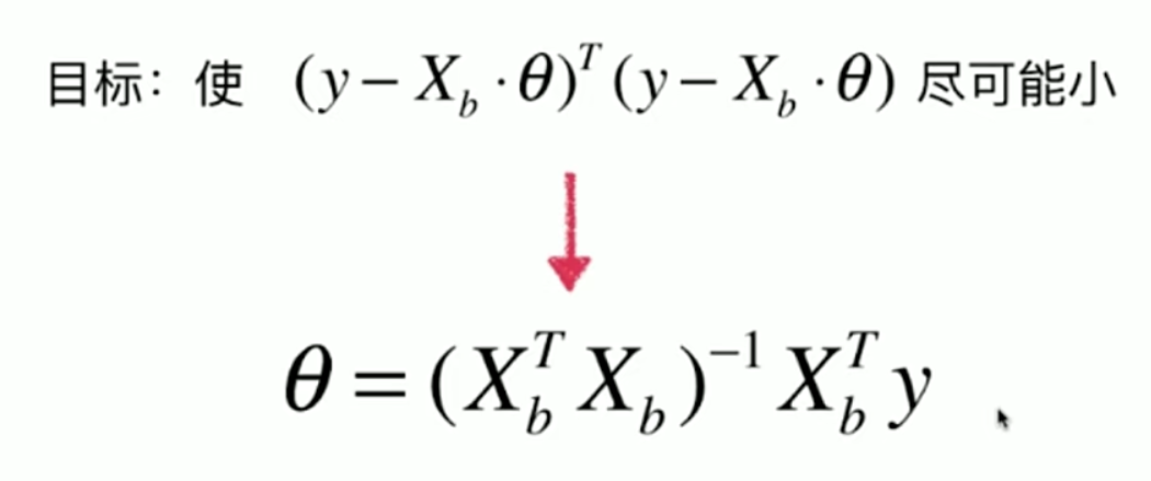
通过矩阵求导计算,可以得到方程解,但求解的时间复杂度很高。
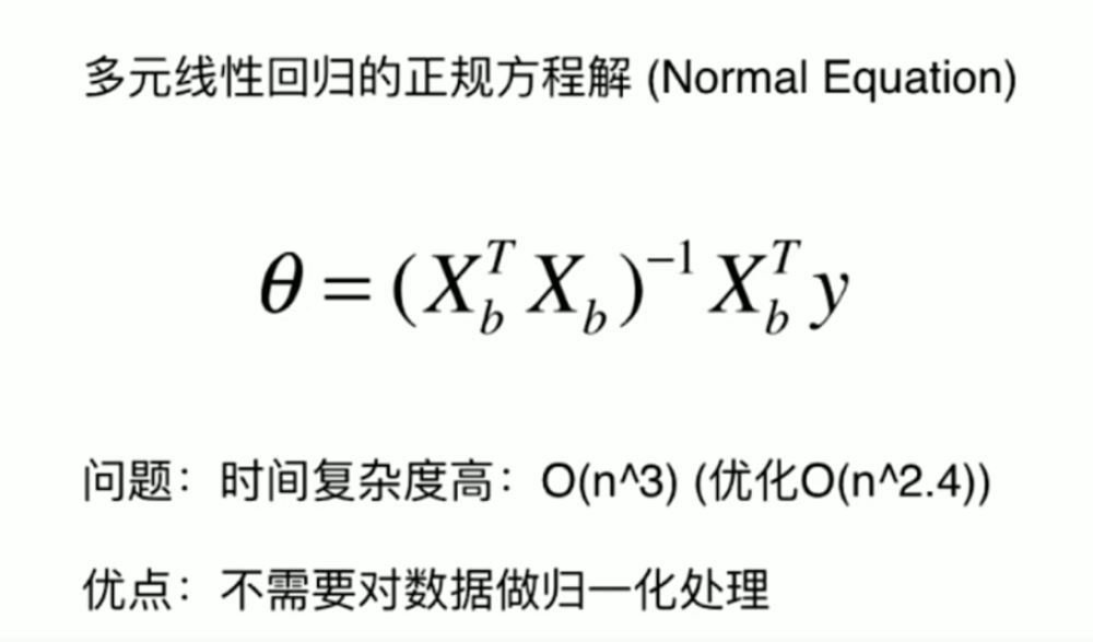
下面使用正规方程解的形式,来对波士顿房价的所有特征做多元线性回归。
import numpy as np
from PlayML.metrics import r2_score
from sklearn.model_selection import train_test_split
import sklearn.datasets as datasets
from PlayML.metrics import  root_mean_squared_error
np.random.seed(123)

class LinearRegression():
    def __init__(self):
        self.coef_=None # coeffient
        self.intercept_=None # interception
        self.theta_=None
    def fit_normal(self, x_train, y_train):
        """
        use normal equation solution for multiple linear regresion as model parameters
        Parameters
        ----------
        theta=(X^T * X)^-1 * X^T * y
        assert x_train.shape[0] == y_train.shape[0],\
            """size of the x_train must be equal to y_train """
        X_b=np.hstack([np.ones((len(x_train), 1)), x_train])
        self.theta_=np.linalg.inv(X_b.T.dot(X_b)).dot(X_b.T).dot(y_train) # (featere,1)
        self.coef_=self.theta_[1:]
        self.intercept_=self.theta_[0]
    def predict(self,x_pred):
        """给定待预测数据集X_predict,返回表示X_predict的结果向量"""
        assert self.intercept_ is not None and self.coef_ is not None, \
            "must fit before predict!"
        assert x_pred.shape[1] == len(self.coef_), \
            "the feature number of X_predict must be equal to X_train"
        X_b=np.hstack([np.ones((len(x_pred),1)),x_pred])
        return X_b.dot(self.theta_)
    def score(self,x_test,y_test):
        Calculate evaluating indicator socre
        ---------
            x_test:x test data
            y_test:true label y for x test data
        y_pred=self.predict(x_test)
        return r2_score(y_test,y_pred)
    def __repr__(self):
        return "LinearRegression"
if __name__ == '__main__':
    # use boston house price dataset for test
    boston_data = datasets.load_boston()
    x = boston_data['data']  # total x data (506,)
    y = boston_data['target']  # total y data (506,)
    # keep data with target value less than 50.
    x = x[y < 50]  # total x data (490,)
    y = y[y < 50]  # total x data (490,)
    # train size:(343,) test size:(147,)
    x_train, x_test, y_train, y_test = train_test_split(x, y, test_size=0.3,random_state=123)
    regs = LinearRegression()
    regs.fit_normal(x_train, y_train)
    # calc error
    score=regs.score(x_test,y_test)
    rmse=root_mean_squared_error(y_test,regs.predict(x_test))
    print('R squared error:%.2f' % (score))
    print('Root mean squared error:%.2f' % (rmse))
输出结果:
R squared error:0.79
Root mean squared error:3.36
1.3 使用sklearn中的线性回归模型
import sklearn.datasets as datasets
from sklearn.linear_model import LinearRegression
import numpy as np
from sklearn.model_selection import train_test_split
from PlayML.metrics import  root_mean_squared_error
np.random.seed(123)

if __name__ == '__main__':
    # use boston house price dataset
    boston_data = datasets.load_boston()
    x = boston_data['data']  # total x size (506,)
    y = boston_data['target']  # total y size (506,)
    # keep data with target value less than 50.
    x = x[y < 50]  # total x size (490,)
    y = y[y < 50]  # total x size (490,)
    # train size:(343,) test size:(147,)
    x_train, x_test, y_train, y_test = train_test_split(x, y, test_size=0.3, random_state=123)
    regs = LinearRegression()
    regs.fit(x_train, y_train)
    # calc error
    score = regs.score(x_test, y_test)
    rmse = root_mean_squared_error(y_test, regs.predict(x_test))
    print('R squared error:%.2f' % (score))
    print('Root mean squared error:%.2f' % (rmse))
    print('coeffient:',regs.coef_.shape)
    print('interception:',regs.intercept_.shape)
R squared error:0.79 Root mean squared error:3.36 coeffient: (13,) interception: ()
加载全部内容